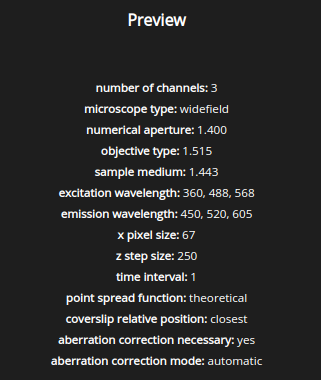
Image template

An image parameter template consists of several microscopic pararameters relevant for deconvolution. To get a preview of the template contents select the template, the contents will be displayed on the right panel.

Note

When editing a template help links are displayed at key locations to point you to specific articles of the SVI-wiki.

Number of channels

Number of fluorescent channels in the image.

Note

Transmission channels can NOT be deconvolved with the algorithms currently available in HRM and should be skipped!

PSF Type

To perform image deconvolution a Point Spread Function (PSF) is needed.

The Huygens software can compute a theoretical PSF from the image parameters used during deconvolution or it can use a measured PSF.

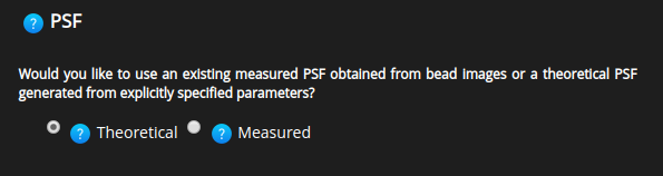
Depending on the user choice HRM will, at a later stage, ask for:

• the path to the file containing the PSF if you selected Measured,

• the settings to correct for spherical aberration if you selected Theoretical and there is a refractive index mismatch.

In most cases a theoretical PSF works fine.

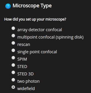
Microscope type

Choose among the supported microscope types: widefield, confocal, spinning disk, multiphoton, STED, STED 3D, SPIM, Rescan, and Array detector (Airyscan). Depending on the Huygens license some of these options might not show.

Note

HRM requires the microscope type as input from the user. HRM will NOT load the microscope type from the selected images automatically.

Import metadata

Some parameters are always present in the meta data of specific file formats and can be imported from the image at run time, while deconvolving the image, to save you time.

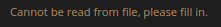
Note

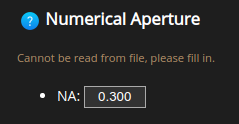
When a parameter is missing from the meta data HRM needs input from the user. This is highlighted by a message like this:

Note

When a parameter is present in the meta data HRM can work without the input from the user. This is indicated with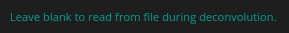

At the end of the deconvolution job, HRM informs on the values of all used parameters as well as their origin (user input or meta data).

Numerical aperture

The Numerical Aperture (NA) describes the amount of light coming from the focus that the objective can collect.

The NA depends on the half angle of the maximum cone of light that can enter or exit the lens. It is directly linked to the resolution of the objective.

Usually, the NA can be found engraved on the objective next to the magnification.

Note

Depending on the selected file format this parameter may be skipped, as explained in Import metadata.

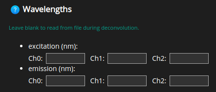
Wavelengths

Excitation and emission wavelengths of each channel. For the emission wavelength the central value of the emission spectrum of the fluorophore can be considered.

Note

Make sure to insert these values in the same order as they were acquired.

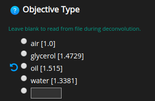
Objective Type

Whether a dry (air) or immersion objective (water, glycerol, oil) was used. For other immersion types it is possible to enter their refractive indexes directly.

Note

Several file formats report this value in the meta data. To leave empty please click on .

Sample medium

Whether glycerol, polyvinyl alcohol, vectashield or water was used to embed the sample.

For other embedding media it is also possible to specify their refractive indexes directly.

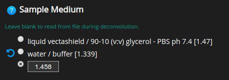
Note

Few file formats report this value in the meta data. To leave empty please click on .

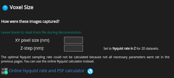
Voxel Size

The voxel size or sampling size is a very important parameter in image deconvolution.

Note

According to the Nyquist criterion its value should not be larger than half the optical resolution of the imaging system.

HRM offers several utilities to help you set up this parameter correctly.

Ideally, the optimal voxel sizes are calculated before acquiring the images. By doing so, one can ensure that the images are compliant with the Nyquist criterion. Click on to determine how large the voxel sizes should be. By using these values, there will be no lost information during the image acquisition and the deconvolution will be able to restore the original signal better.

If the optimal voxel sizes have not been determined before the acquisition stage one can calculate the resulting sizes in widefield and spinning disk microscopy by using . Here the voxel sizes are calculated from the CCD camera element, the objective magnification, etc., although no optimal voxel size can be guaranteed.

Note

Make sure to set a voxel size consistent with the Nyquist criterion. Undersampled images will often show artifacts after deconvolution.

Lastly, for deconvolving time series set the time interval between subsequent frames.

Among other things, this will help HRM to decide when to stabilize the image.

Using a measured PSF

This option will only appear if ‘measured PSF’ was selected as PSF Type in a previous step.

Distilled PSFs need to be created beforehand using Huygens Professional and uploaded to the Raw images folder.

Note

One PSF image per channel. Multichannel PSFs are not supported.

When presented with the Distilled PSF file selection window,

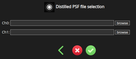
browse for the distilled PSF appropriate for the channel(s) of the image.

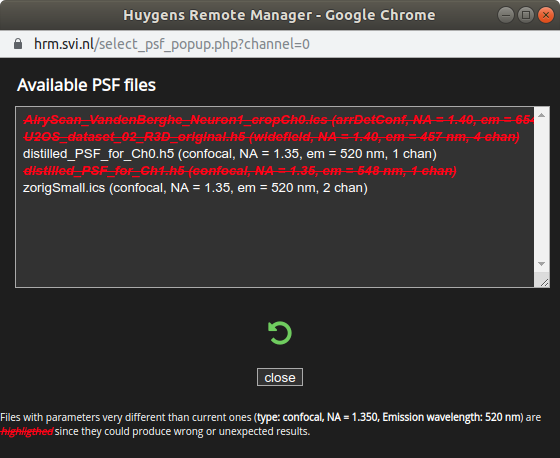
Select the PSF file and click close. Repeat for all channels.

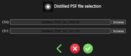
Afterwards, press save and return to the image parameter selection page.

Note

Files that can’t work as PSFs for the selected image(s) are crossed off and displayed in red.

Pinhole Radius

Pinholes are used in confocal, spinning disk, STED, STED 3D and Rescan microscopy to get rid of out-of-focus light. Since there’s no pinhole in widefield, two photon and SPIM microscopes HRM skips this parameter in those cases.

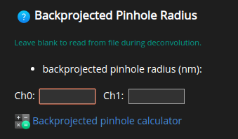
Note

HRM needs the value of the pinhole backprojected on the specimen.

Further help on how to calculate the backprojected pinhole radius can be found on .

Pinhole Spacing

Spinning disk microscopy uses more than one pinhole to speed up image acquisition. The backprojected distance between these pinholes also plays a role in image deconvolution. HRM skips this parameter for all other microscope types.

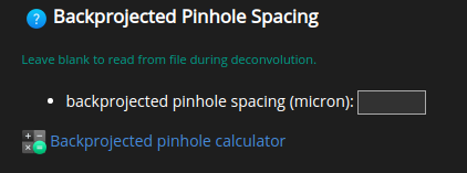
Click on for further help on the calculation of the backprojected value.

STED parameters

If the selected microscope type is STED or STED 3D then a few STED parameters need to be specified to describe the STED acquisition. When working with other microscope types HRM will skip these parameters.

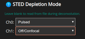
First, select the STED depletion mode: Pulsed, Continous wave gated detection, Continous wave non gated detection or Off/Confocal.

Note

STED and confocal microscopy are often combined. That’s why even if the selected microscope type is STED it’s still possible to set specific channels as confocal at this point.

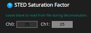
Set the STED saturation factor of each channel. Typical values are in the range of 10 to 50. The higher this factor, the more suppression of fluorescence away from the optical axis, the more resolution.

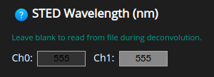
Next, set the STED depletion wavelength of each channel. Notice that Channel 1 is grayed out in these figures because it was set as confocal.

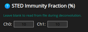
The STED immunity fraction tells Huygens the percentage of fluorescent molecules that are not susceptible to the STED laser. Typical values are in the range 0% to 10%.

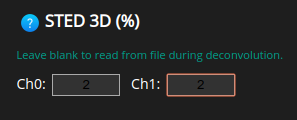
Finally, depending on whether the microscope type is STED 3D or not, set the percentage of STED 3D per channel. This tells Huygens how much power was used in the Z depletion beam. The remaining power is used for the vortex path.

SPIM parameters

If the selected microscope type is SPIM then a few SPIM parameters need to be specified to describe the SPIM acquisition. When working with other microscope types HRM will skip these parameters.

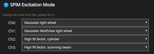
First, select the SPIM excitation mode of each channel: Gaussian light sheet, Gaussian MultiView light sheet, High fill factor (cylinder), or High fill factor (scanning beam).

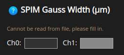
Set the width of the Gaussian light sheet for the channels acquired with one of the Gaussian modes. The field will be grayed out for the other channels.

The width is defined as the distance between the two (symmetric) points of the Gaussian profile where the intensity values drop to 2/e^2 of the peak value.

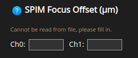
Set the SPIM Focus Offset of the light sheet. This is the distance along the optical axis of the detection lens between the focus of the illumination lens and the focus of the detection lens.

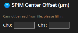
Similarly, set the SPIM Center Offset of the light sheet. This is the distance along the optical axis of the illumination lens between the focus of the illumination lens and the focus of the detection lens.

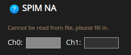
Set the SPIM NA for the channels aquired with the one of the High Fill Factor modes. This is the Numerical Aperture of the illumination lens.

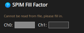
Then, the fill factor of the illumination lens, for the channels acquired with one of the High Fill Factor modes. This is the ratio between the beam width and the diameter of the objective pupil in the illumination lens.

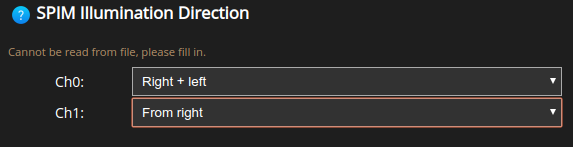
Lastly, the SPIM Illumination Direction. This can be left, right, bottom, top for any of the non-MuVi (Multi-View) excitation modes; and right+left or top+bottom for the Gaussian MuVi excitation mode.

Spherical Aberration correction

Spherical aberration is mainly caused by a mismatch between the refractive indexes of the objective immersion medium and the sample embedding medium.

HRM will automatically detect this mismatch and ask whether the aberration should be corrected for when using a theoretical PSF.

Note

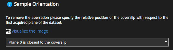
Spherical aberration can be corrected for by creating different theoretical PSFs (with slightly changing shapes) at different depths: depth-dependent PSF.

When using a depth-dependent PSF one also needs to specify whether the first plane in the dataset is closest or farthest to/from the coverslip.

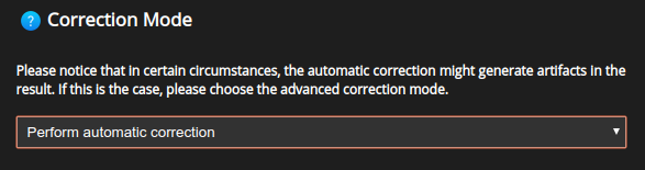
The Correction mode allows for a more detailed choice as to how the depth-dependent PSF should vary with depth.

• Automatic correction: will generate a depth-dependent PSF where the PSF is automatically selected at each depth, as explained above.

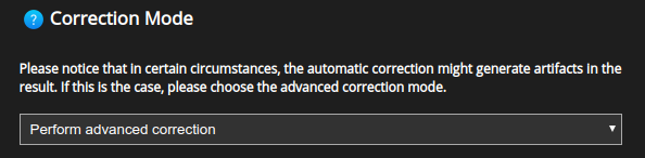
• Advanced correction: allows to specify further details about the depth-dependent PSF.

The Advanced correction will further enable a number of advanced options.

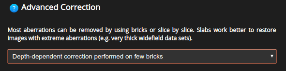
• Depth-dependent PSF on few bricks: a different PSF will be generated for each Z brick in which the original data is split.

• Depth-dependent PSF slice by slice: a different PSF will be generated for each slice.

• Depth-dependent PSF on few slabs: several PSFs will be generated for each Z brick. This option is memory-consuming but the best choice when the spherical aberration is very strong.

Note

Splitting the original data into bricks while deconvolving not only helps to correct for spherical aberration but it also minimizes the amount of RAM memory needed for deconvolution.